
[ 딥러닝 ] Recurrent Neural Networks - part 2
Updated:
short-term dependency vs. long-term dependency
short-term dependency
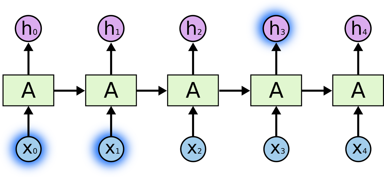
- 근처 시점의 데이터와의 관계
- 필요한 정보를 얻기 위한 시간 격차가 크지 않은 경우이다.
long-term dependency
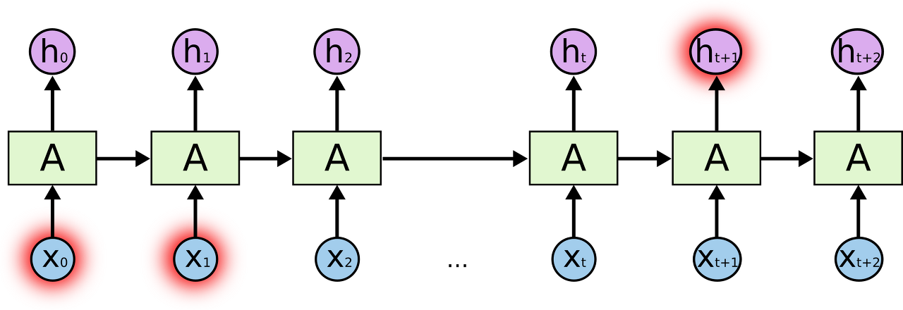
- 멀리 있는 시점의 데이터와의 관계
- (vanilla) RNN은 long-term dependency에는 약하다는 것이 본질적인 한계점
- RNN의 특성
input sequence의 길이에 따라 hidden layer 계산이 반복된다. 그런데 굉장히 길이가 긴 input sequence를 사용하는 것이 상당수이다.
- input sequence의 길이가 길면 sequence 앞부분 요소의 영향력은 time step이 진행될수록 점점 약해져 ($w<1$이면 exponentially decay) 나중에는 소멸할 것이다.
weight sharing을 하므로 timestep 방향으로 backpropagation을 할 때 동일한 weight가 gradient에 반복적으로 곱해진다.
- gradient vanishing / exploding 발생…!
- RNN의 특성
BPTT (backpropagation through time)
- RNN의 backpropagation 방식
BPTT 방식
먼저 아래와 같이 Gradient Descent 방식으로 weight를 업데이트할 수 있으며, 전체 loss function은 각 시점 t에서의 loss function를 더해서 구할 수 있다.
\[\begin{align*} & W_{hh} ← W_{hh} - \alpha \frac{\partial \;Loss}{\partial W_{hh}} \\ \, \\ & Loss = L(x,y,W_{hh},W_{hy}) = \sum_{t=1}^T \ell(y_t,o_t) \end{align*}\]- $x$, $y$ : 전체 input, output
- $\ell(y_t,o_t)$ : 각 시점 $t$에서의 loss function
- $y_t$ : 시점 $t$에서의 정답
- $o_t$ : 시점 $t$에서의 예측값 (= $\hat{x}_t, y_t$)
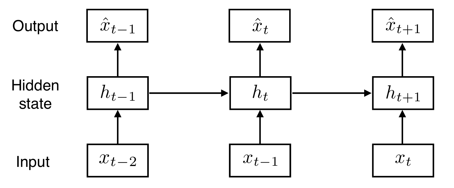
그리고 이와 별개로 각 시점 $t$의 latent vector $h_t$, output $o_t$은 다음과 같이 표현할 수 있다.
$h_t=f(x_t,h_{t-1},W_{hh})$
- latent vector $h_t$는 현재 input $x_t$, 이전 시점의 latent vector $h_{t-1}$ 그리고 hidden-hidden 간의 weight $W_{hh}$에 대한 함수이다.
$o_t=g(h_t,W_{hy})$
- output $o_t$는 현재 latent vector $h_t$, hidden-output간의 weight $W_{hy}$에 대한 함수이다.
이제 chain rule을 이용하여 loss function의 gradient를 표현하면 다음과 같다.
\[\begin{align*} \partial_{W_{hh}} L(x,y,W_{hh},W_{hy}) &= \sum_{t=1}^T \partial_{W_{hh}} \ell(y_t,o_t) \\ \, \\ &= \sum_{t=1}^T \partial_{o_t} \ell(y_t,o_t) \; \partial_{h_t} g(h_t,W_{hh}) \; [\partial_{W_{hh}} h_t] \end{align*}\]$\partial_{o_t}\ell(y_t,o_t)$
- 현재 시점 $t$에서의 loss function을 output $o_t$에 대해 편미분한 것
$\partial_{h_t}g(h_t,W_{hh})$
- 현재 시점 $t$에서의 output을 latent vector $h_t$에 대해 편미분한 것
$\partial_{W_{hh}}h_t$
- 현재 시점 $t$에서의 latent vector를 hidden-hidden 간의 weight $W_{hh}$로 편미분한 것
여기서 각각의 latent vector $h_t$는 이전까지의 latent vector $h_{t-1},h_{t-2},…,h_1$에 대해 의존적이기 때문에 이를 고려할 필요가 있다. 그러므로 $\partial_{W_{hh}} \ell(y_t,o_t)$는 다음과 같이 풀어 쓸 수 있다.
\[\begin{align*} &\partial_{W_{hh}} \ell(y_t,o_t) \\ \, &= \partial_{o_t} \ell(y_t,o_t) \; \partial_{h_t} g(h_t,W_{hh}) \; [\partial_{W_{hh}} h_t] \\ \, &= \partial_{o_t} \ell(y_t,o_t) \; \partial_{h_t} g(h_t,W_{hh}) \; \{ \partial_{W_{hh}} h_t + \partial_{h_{t-1}} h_t\,\partial_{W_{hh}}h_{t-1} + ...\} \end{align*}\]$\partial_{W_{hh}}h_t$
- $h_t$만 고려해서 현재 latent vector $h_t$를 $W_{hh}$로 편미분한 것
$\partial_{h_{t-1}} h_t\,\partial_{W_{hh}}h_{t-1}$
- $h_{t-1}$ (한 시점 이전)을 고려해서 $h_t$를 $W_{hh}$로 편미분한 것
$\partial_{h_{t-1}} h_t\,\partial_{h_{t-2}} h_{t-1}\partial_{W_{hh}}h_{t-2}$
- $h_{t-2}$ (두 시점 이전)를 고려해서 $h_t$를 $W_{hh}$로 편미분한 것
여기서 latent vector의 한 시점 이전 latent vector에 대한 변화량인 $\partial_{h_{t-1}} h_t,\;
\partial_{h_{t-1}} h_t\,\partial_{h_{t-2}} h_{t-1},…$ 항은 sequence가 길어질수록 불안해지기 쉽다.
→ gradient vanishing 문제 발생!